OpenCV: comparing the speed of C++ and Python code on the Raspberry Pi for stereo vision

You often hear that Python is too slow for computer vision, especially when it comes to single-board computers like Raspberry Pi. Python is very simple and easy to learn, and it’s currently one of the most popular programming languages for a good reason.
So how good Python’s performance in computer vision tasks actually is? Where exactly is it slower than C++, and how much? The answer to this question is not so clear. For example, when constructing depth maps on Raspberry Pi using Python code, it uses binary libraries written in C++ ‘under the hood’. They are perfectly optimized specifically for the raspberry processor (Neon and all that), and this code works very fast!

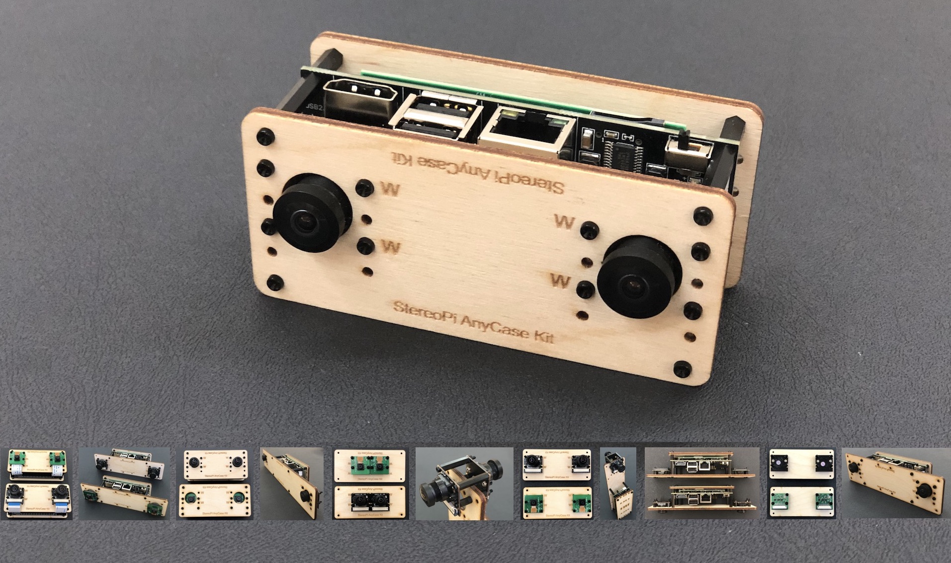
In this article, we decided to measure the actual speed difference and find the performance 'bottleneck'. The approach is very simple. We have a series of small Python programs that allow you to go through all the stages from the first launch of the stereo camera and its calibration to building a depth map from real-time video (and a 2D space map in a mode that emulates the operation of a 2D lidar). We ported all this code to C++, and we compare performance at each stage. For hardware we used the Raspberry Pi Compute Module 3+ Lite installed on a StereoPi expansion board.

Before we begin

We live in the era of Twitter, Instagram and other short message services. Therefore, for ease of perception, we divided the article into two sections. The first one is a brief and concise overview of the experiments and performance. The second one – a detailed analysis of all the steps taken and of the bugs found, which will be interesting to those who’d like to repeat the experiments.

Let's get started!

So, we have a StereoPi stereo camera based on the raspberry Pi Compute Module 3+, and we want to get a depth map from real-time video. To do this, we need to go through several steps:

• Assemble the device and verify that everything is working correctly
• Make a series of pictures for calibrating the stereo camera
• Calibrate the stereo camera using the pictures taken
• Configure the depth map settings
• Get the depth map from the video in real time
• Get a 2D space map in real time

For each of these steps, we have ready-made scripts in Python and the same scripts ported to C++. On GitHub, the Python scripts live here, and the C++ ones live here.

Script 1 – testing video capture speed

At this stage, we simply capture stereoscopic video from the cameras and display it on a screen. In Python, we use the PiCamera library for this, and in C++ we use the pipe transfer from the fastest of native applications, namely raspividyuv. Details can be found below in the 'Detailed Debriefing' section.

C++ code
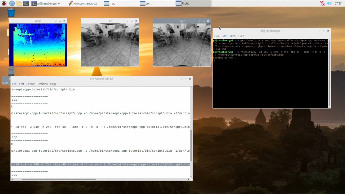
Here how the compilation and launch procedures look on the screen:

Compile the example, and first run the code with a stereo resolution of 640x240, that is with two 320x240 pictures.
Compile:

g++ /home/pi/stereopi-cpp-tutorial/src/script1.cpp -o /home/pi/stereopi-cpp-tutorial/bin/script1.bin -I/usr/local/include/opencv4 -L/usr/local/lib -lopencv_core -lopencv_highgui -lopencv_imgcodecs -lopencv_imgproc -lopencv_calib3d

Run:

raspividyuv -3d sbs -w 640 -h 240 -fps 30 --luma -t 0 -n -o – | /home/pi/stereopi-cpp-tutorial/bin/script1.bin

Quit the script using the Q key and you should see this output:

Average FPS: 30.3030
Let's try to output 90 FPS.

raspividyuv -3d sbs -w 640 -h 240 -fps 90 --luma -t 0 -n -o – | /home/pi/stereopi-cpp-tutorial/bin/script1.bin

Output:
Average FPS: 90.90

So where’s the limit? Let’s set 150 FPS:

raspividyuv -3d sbs -w 640 -h 240 -fps 150 --luma -t 0 -n -o – | /home/pi/stereopi-cpp-tutorial/bin/script1.bin

Average FPS: 90.909088 Well then, the limit is 90 FPS. Not bad.

Now let's try capturing at a higher resolution. To do this, make two changes:

• In the code, specify the resolution of 1280x480
• In the raspividyuv parameters, specify the resolution of 1280x480

Compile and then run with the following parameters:

raspividyuv -3d sbs -w 1280 -h 480 -fps 90 --luma -t 0 -n -o – | /home/pi/stereopi-cpp-tutorial/bin/script1.bin

The result is 39 FPS.
We ran this code with different FPS, and this is what we got: 

Resolution	FPS requested / achieved	FPS requested / achieved	FPS requested / achieved	Optimal FPS  settings
640x240	250 / 90.9	150 / 90.9	90 / 90.9	Up to 90
1280x480	150 / 43.5	90 / 43.47	45 /45.5	Up to 40

 

Please note that if you set FPS a bit higher than recommended, you'll see noticeable lag and lost frames in the preview.

Python code
Here is how the script works:

So, we’re trying to capture a 768x240 picture, setting the desired FPS at 30. (See the 'Detailed debriefing' section for why the resolution is set at this value)

Go to the stereopi-fisheye-robot folder, and run:

python 1_test.py

You’ll see that when there’s movement in the frame the picture 'stutters' a lot, and after stopping the script the average FPS is 9.75

Hmm, the result is not very good. We requested 30, but we got 9.7 FPS. But there is a catch. Unlike the C++ solution, Python is much more sensitive to correct FPS configuration. If you request substantially more than necessary, you’ll get not the maximum available FPS, but a sharp drop in FPS.

Let's capture our picture at 20 FPS.
Output: FPS 20.8211

Now we’re talking! We doubled the capture efficiency by indicating the correct FPS for this particular situation.
Here is a brief summary of the requested and achieved FPS for our script number one:

Resolution (side-by-side stereo)	FPS requested / achieved	FPS requested / achieved	FPS requested / achieved	Optimal FPS  settings
768x240	50 / 7.99	30 / 9.44	20 / 20.8	20
1280x480	50 / 5.65	30 / 5.26	20 /15.4	15
640x240 (scaled by GPU from 1280x480)	50 / 6.1	30 / 13.94	20 / 19.96	20

 

Final comparison of frame capture speed with C++ and Python code with the respective recommended settings:

	1280x480 (stereoscopic)	640x240 (stereoscopic)
C++	40 fps	90 fps
Python	15 fps	20 fps

 

Script 2 - checkerboard session

In the second stage, we take a series of pictures with a checkerboard for subsequent calibration. There’s no need to compare performance here, since saving series of snapshots every 3-5 seconds is not difficult for either C++ or Python code. 
Only two differences can be noted for this stage:

• The C++ code shows a BW picture 
• The C++ code allows you to show a photo preview window with a higher FPS

Otherwise, there is no difference between the scripts.

Compiling and running the example in C++:

Running the Python code:

 

Script 3 – slicing image pairs

This script has a very simple logic, so we didn’t make it into a separate C++ binary, but added its functions to the previous code example. 
Therefore, with our C++ code you can immediately go to script 4, and with the Python code you need to run 3_pairs_cut.py to slice the pictures into pairs. We showed the slicing process with the Python script at the end of the previous video.
To avoid experiment bias in our further measurements, we copied all the images (the scenes folder) taken using C++ code into a similar Python script folder, and then ran the slicing script. This way, both solutions will work with the same set of images.

Script 4 – Calibration

Let's start with the results:

• Python: 17 seconds importing (and searching for the checkerboard), 13 seconds calibrating
• C++: 19 seconds importing, 9.27 seconds calibrating

As you can see, Python imports pictures a little faster, and C++ code performs calibration faster. But overall performance is roughly equal. The interesting bit is that the same code with the same settings has different efficiency in finding the checkerboard on images (Python turned out to be better at this). Details, as agreed, come in the second section of this article.

Video of the C++ calibration code at work

Video of the Python calibration code at work

 

Script 5 – setting the parameters of the depth map

At this stage, we configure the parameters of the depth map so that its quality suits us. 
Looking ahead, I’ll just say that the comparison here is not in favor of Python. We used the matplotlib library to display the depth map in Python. It’s flexible, convenient, but not designed to display rapidly changing data in real time. Therefore, it takes almost a full second from the moment you change any parameter until the updated depth map is displayed. And we use only one static image for the settings.
But in C++ our hands are untied, so we were able to make settings adjustments with real-time video. 

Here’s how it looks in Python:

And how it looks in C++:

Script 6 – depth map from video

So, we’ve come to one of the most interesting parts – code speed in applied tasks.
Here's how it works in Python code. To avoid making the next video boring, we first ran the script with the usual parameters to show the common problem of 'jumping colors' on the depth map, and then we turned on auto color adjustment and looked at the depth map again.

In the process, the script displays the average time it takes to build each depth map. You’ll see that it varies from 0.05 to 0.1 seconds. As a result, you get approximately 17 FPS. Please note that FPS may depend on your depth map calculation settings!

And now the same task, but in C++:

The average result is also about 17 FPS.

A couple of conclusions:

1. Both the Python and the C++ codes yield approximately the same performance when calculating depth maps. As mentioned at the beginning of this article, for these calculations Python calls binary libraries that are very well optimized for the Raspberry Pi processor.
2. Despite the fact that C++ is capable of capturing video at much higher FPS, this advantage becomes meaningless, since the system doesn’t have enough time to calculate depth maps at the speed needed.

 

Script 7 – 2D space map in scanning lidar mode

The idea of ​​this script is very simple. We’ll build a depth map not from the entire image, but only from a part of it – a horizontal strip in the center of the image, a third of the entire frame’s height. In this case, the operation of the stereo camera is more similar to the operation of a scanning rangefinder. By changing the height of this strip, you can adjust the sensitivity of the system. After getting a depth map, we project it onto a plane and get a two-dimensional obstacle map for the robot.

Here's how the Python code works:

And here's the C++ version:

 

A conclusion from these tests. We calculate the depth map only from a part of the image, which reduces the load and increases the FPS of the resulting map. But for Python code, this doesn’t yield a performance gain since the bottleneck is in the process of capturing frames – our code cannot do it faster. But the C++ code has a margin in video frame capture speed (up to 90FPS), which yields quite a boost. I can only say that the speed significantly exceeds 30 maps per second. We’ll leave exact measurements to our readers. ☺

Final conclusions on Python and C++ performance comparison

In most of the considered examples, C++ code is much faster, but in the key task – calculating depth maps from video – the performance of both solutions is the same. The bottleneck is in the peak CPU performance when calculating depth maps (a little less than 20 FPS in both C++ and Python). So for those who are beginning to study computer vision, Python is a great fit.

And the second conclusion. The bottleneck of the current Python code is the video frame capture speed. Fortunately for us, the frame capture efficiency is roughly equal to the depth map calculation efficiency (about 20 frames per second in both cases). But we left a few loopholes for those who need more speed when capturing frames.

What can be improved?

Actually, in Python you can use a capture method similar to that used in C++ code – transferring video through a pipe with the speedy raspividyuv utility. The second approach is the solution proposed by the author of PiCamera in one of his answers on Raspberry.stackexchange. 

The binary code for calculating depth maps does not implement multithreading, therefore, approximately one and a half cores out of four are used in the process. Theoretically, there’s margin for a twofold speed increase in building depth maps.

Section 2 – Detailed debriefing

Preparing the Raspbian image
So, let’s get straight to business.

• OpenCV 4.1.0 for use with C++ was compiled from source following instructions on pyimagesearch.com. Answers to most questions about errors that may arise can be found in the comments to that article.
   
• We added additional swap partitions to successfully compile OpenCV from source. Our Raspbian image also has them, so you can completely rebuild OpenCV if necessary.
   
• OpenCV versions:
  C++ – version 4.1.1
  Python – version 4.1.0 (installed via pip)
  By default Python 3 is used (bindings call python3 when running python).
   
• To enable support for the second camera, just put our dt-blob.bin in the /BOOT folder. This file is already present in our image.
   
• In the latest Raspbian kernels stereo mode support was broken accidentally. The reason is the new white balance algorithm. Thankfully, a Raspberry Pi Foundation engineer proposed a solution – switch AWB to the old mode, and stereo will work again. We added the switch command (sudo vcdbg set awb_mode 0) to  /etc/rc.local, and it’s executed automatically every time the system boots.
   
• raspividyuv received video support relatively recently, and it’s not available in the latest versions of Raspbian available for download (as of January 2020). To enable stereo, you need to run sudo rpi-update.
   
• After the rpi-update or even a full apt-get upgrade, an error occurs causing the file manager to close itself immediately after opening. It turns out that Buster has updated the interface. This can be cured with a full-upgrade command.
   
• About code versions. Currently, our most popular repository is stereopi-tutorial. Actually, the new stereopi-fisheye-robot repository used in this article is a more recent version, which we’ll base further development on. In addition to supporting more recent versions of OpenCV, it supports fisheye cameras and removes dependencies on external calibration libraries. All the code works perfectly fine with regular (not fisheye) cameras too.

Script 1 – video capture

C++ and video capture caveats

• To capture video in C++, you can use the low-level MMAL API. The main applications raspivid, raspividyuv and others from this group were written using this particular API. The source code for them can be found on GitHub. We wanted to keep Python and C++ code as close as possible, so we did not complicate the program by using these functions. 
• We took the fastest native video frame capturing application – raspividyuv. Moreover, we decided to get the most out of it by tweaking settings. The depth map is built from a BW picture, and you don’t need color for that. The --luma option used in our launch commands allows you to transfer only the alpha channel, or the black and white component of the image. This way, we pass 3 times less data to our program than it would have taken to transfer a color picture.
• Our video from raspividyuv comes in RAW format. The receiving side cannot figure from the data it gets where one frame ends and another one begins. Therefore, if you specify one resolution on the receiving end and another one in raspividyuv, incidents like this one are bound to happen:

Python and video capture caveats
The first thing you need to know is that PiCamera is very cool! In the well-written documentation you can find a lot of unique information about the peculiarities of the Raspberry Pi video system (which cannot be found anywhere else!), and I recommend reading it before going to sleep. ☺ Just take a look, for example, at the Advanced recipes section!
Using various sources of information, we collected the following requirements for image resolution, which don’t cause trouble during capture:

• the height of the final image should be a multiple of 16
• the width should be a multiple of 32
• the width of each image in a stereo pair must be a multiple of 128

Scary, huh? Here is an example of a picture captured with incorrectly set parameters:

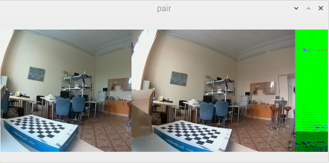
Here we tried to capture a stereo picture with a resolution of 640x240 (two frames of 320x240 each). But 320 is not a multiple of 128. You can see that the frame from the left camera is narrower (256 pixels), while the right one is of normal width (320 pixels). 
No reason to be scared though. There are two ways around this:

• either set the resolution according to the rules – 384x240 for each frame (or 768x240 for the stereo image)
• or capture a higher resolution and reduce it to the required parameters via the GPU (this actually solves a lot of problems). In our code, we capture at 1280x480, and then halve the picture (the scale_ratio value is set to 0.5 on line 48 of the first Python script). We recommend this method, as it greatly simplifies life (and, by the way, doesn’t put additional load on the processor). 

We repeat here a part from the first section of this article. Actually, in Python, you can use a capture method similar to that used in C++ code – transferring video through a pipe with the speedy raspividyuv utility. The second approach is the solution proposed by the author of PiCamera in one of the answers on Raspberry.stackexchange (the numpy.frombuffer method without copying extra data in memory).

Script 4 – Calibration

Lifehack
First, a few words about a lifehack that greatly improves the search for the checkerboard in the image. We need to calibrate for a resolution of 320x240, but the checkerboard detection is poor for pictures of this resolution. Therefore, we take pictures at double the resolution (640x480), find the checkerboard corners’ coordinates on them, and then reduce the coordinates by half on the X and Y axis. And only then feed them to the calibration mechanism. If you need even higher accuracy, you can calibrate at 1280x960 and then reduce the coordinates found by 4 times.

Same can be different
Here’s an interesting observation – using the same search parameters for the checkerboard, the Python code finds it on more images. You must have noticed on the video that Python throws away just one pair where it didn’t find the checkerboard, while C++ discards a dozen. Most of the pictures where the checkerboard wasn’t found are photos where the checkerboard is at a great distance from the camera. I see no other explanation than the difference in the OpenCV 4.1.1 and 4.1.0 algorithms (the former version is used in C++, and the latter in Python).  

Bugs while calibrating on Python
If you start calibration with all the pictures in the examples, the calibration fails with an error:

Traceback (most recent call last):
File "/home/pi/stereopi-fisheye-robot/4_calibration_fisheye.py", line 297, in <module>
result = calibrate_one_camera(objpointsRight, imgpointsRight, 'right')
File "/home/pi/stereopi-fisheye-robot/4_calibration_fisheye.py", line 170, in calibrate_one_camera
(cv2.TERM_CRITERIA_EPS+cv2.TERM_CRITERIA_MAX_ITER, 30, 1e-6)
cv2.error: OpenCV(4.1.0) /home/pi/opencv-python/opencv/modules/calib3d/src/fisheye.cpp:1372: error: (-215:Assertion failed) fabs(norm_u1) > 0 in function 'InitExtrinsics'

This is a very unpleasant error, and the difficulty in understanding the logic of its appearance makes it even worse. Actually, in this case, it is caused by picture 23, even though this picture looks quite good, the checkerboard is perfectly visible on it, and nothing portends trouble. The only way to get rid of this error is to find and remove the problematic picture. I use the ‘division in half’ method for this.
Let's say we have 50 images for calibration. I delete 25 pictures and see whether the error persists. If it disappeared, I leave these pictures and return half of the deleted ones (12 or 13). If the error appears again, I delete them again, but return the other half. Further on, it’s already work with half of a half  – 6 or 7 pictures. Then I repeat this with 3 pictures, and finally find the culprit. As far as we were able to understand, it’s not the picture itself that is at fault, but rather the correlation of its parameters with the other pictures in the set. In some cases, images with a different number may become problematic – for example, if you start calibration from image 1 and then add others one at a time.

Bugs while calibrating on C++
The presence of picture 47 in the calibration series causes this error:

terminate called after throwing an instance of 'cv::Exception'
    what(): OpenCV(4.1.1) /home/pi/opencv/modules/calib3d/src/fisheye.cpp:1421: 
error: (-3:Internal error) CALIB_CHECK_COND – Ill-conditioned matrix for input array 37 in function 'CalibrateExtrinsics'

Aborted

Image 47 was found using the ‘division in half’ method, as was the case with the Python code (where picture 23 was misbehaving).
It’s worth noting that there is a hint in the error itself – the problem is in the input array #37. This is a great achievement, since in previous versions of OpenCV you didn’t even get this information.
You can see that the error was caused by processing with the flag CALIB_CHECK_COND, which was definitely not explicitly set. If you try to clear this flag explicitly (on the commented out line //fisheyeFlags &= cv::fisheye::CALIB_CHECK_COND), you get another error:

terminate called after throwing an instance of 'cv::Exception'

  what(): OpenCV(4.1.1) /home/pi/opencv/modules/calib3d/src/fisheye.cpp:1023: error: (-215:Assertion failed) abs_max < threshold in function 'stereoCalibrate'

Aborted

As with the Python code, the cause is in one image, and removing it from the list of processed images solves this problem.
Well, what can I say here – this is a very user unfriendly situation. It would be logical to implement, for example, ignoring erroneous arrays instead of stopping work altogether (as an additional flag), or give users a tool to pre-validate the array before sending it for calculation. But for now we’re left only with ‘sifting’ the pictures through ‘division in half’ (or editing the OpenCV code and rebuilding it completely from scratch). We hope that this issue with calibration will be fixed in the next releases of OpenCV.

Script 5 – configuring the depth map

Our implementation of the settings interface in C++ has a ‘twisted’ issue – the min_disp parameter can be negative while the slider in our interface starts from zero. Therefore, we subtract 40 from the value on the slider to capture the negative range. So 0 on the scale actually means -40 in parameters.
While playing with parameters in C++, you can see the current FPS in the console (more precisely, the DMPS – Depth Maps Per Second). This way, it’s easy to determine which parameters and how affect the speed of calculating depth maps.

Script 6 – depth map from video

About speed. After launching the depth map, look at the processor load with the top or htop command (the latter will show loads per core). You’ll see that usually about one and a half cores are under load. The current Depth Map implementation doesn’t support multithreading (which is still possible in the code). This means that we have approximately two times the potential performance margin, but achieving it requires serious editing of the OpenCV source code.

Script 7 – building a 2D space map in scanning lidar mode

Most of the tricks in this code involve displaying the map on the screen. In some cases, images can be discarded when points on a 2D map are far from the camera. In this case, the automatic scale changes so that the map becomes very small. In this case, we left the option to turn off automatic scaling so you can set one that is most suitable for your particular case. It’s worth noting that with live use on the robot this problem disappears, since you don’t need to display the map, but only need to do the necessary calculations.

Depending on the position of the camera on the robot, you can change the settings of the cut-out image strip by moving it higher, lower or changing the height. And if your StereoPi is connected to a position in space sensor (IMU), then the possibilities of using the resulting map expand dramatically. But here we venture beyond the scope of the article (and touch on the subject of ROS).
 

Links:

Python code: GitHub, stereopi-fisheye-robot
C++ code: GitHub, stereopi-cpp-tutorial
Raspbian image:  Buster, Python and C++ code included